Locating and Operationalizing the Analytic Horizon

In the previous post, Miguel explored simpleA.mdl as an introduction to a technique for agent-based modeling based on constructivist identity theory. This model consists of 2500 agents, each with an activated identity and a repertoire of five other subscribed identities. As the model runs, agents are able to activate new identities from within their repertoire, trade identities within their repertoire for other identities present in the landscape and even activate on identities present in the landscape but not present in the agents repertoire at the time. If you watch simpleA.mdl run, you can observe this behavior as agents assess their environment, decide what identities are available to them (as dictated by their identity repertoire and the triggers that determine under what conditions an agent will rotate their activated identity, substitute a new identity for a subscribed identity, or activate a new identity from outside the agents' repertoire), and activate on the optimal identity.


However, you will also notice that after twenty or thirty timesteps the model reaches an equilibrium where all agents are activated on the optimal identity given their neighborhood. The problem with this is that the equilibrium state does not reflect our understanding of the world, which seems to be in a constant state of flux. There may be periods of stability, but at any level of society a permanent state of equilibrium is virtually unimaginable. One reason for the disconnect between SimpleA.mdl and our understanding of how the world works is a function of the inability of modelers, of any type, to know everything there is to know about the inputs required to make an accurate model. No matter the subject, there is always a vast array of information that would be impossible for us to know and therefore impossible for us to model precisely. In other words, there is always more information beyond the analytic horizon.

One very tangible example of this concept of an analytic horizon is the answer to a seemingly simple question: What is the length of the coast of Britain? The answer however is impossible to determine pr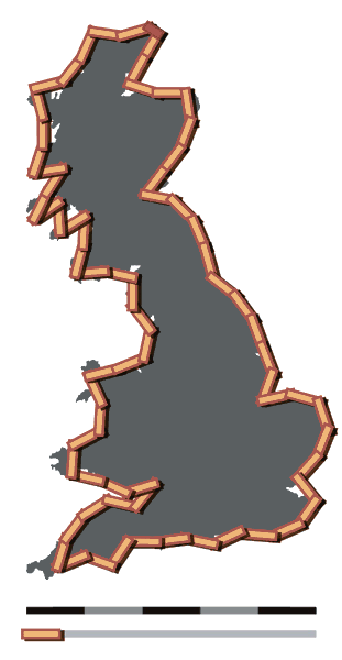ecisely. What is your metric for measuring the coastline? In the image on the left, measurements are taken using 200km as the base unit which means the coastline of Britain is ~2400km long. The image on the right uses a base unit of 50km meaning the coastline of Britain is ~3400km long. One might think that this problem can be solved simply by using more precise measurements, but this is an unrealistic option. It is possible to measure the coastline of Britain using a base unit of 1km and you will find the coastline is much longer than with a unit of 50km. You could then use a base unit of 1cm and the coastline will be even longer. What happens when the unit of measurement is small enough to be operating on a molecular level? Are gaps between atoms measured as coastline? Ultimately, the question of how long the British coastline is can only be answered by explicitly dictating what level of analysis you will be working with, in other words, where the analytic horizon is.

In terms of our PS-I models, we've decided to model the identity composition of a given landscape and the rules by which agents activate and transfer identities. Any other information about the world that plays a role in identity politics lies beyond our analytic horizon. One of the most important characteristics of identity politics that lies beyond our analytic horizon is societal perception of identity. For any number of reasons, one identity could become more favorable than another identity at any given time. Perhaps an individual representing a political party has been involved in some sort of scandal that reflected negatively upon the whole party, or an outbreak of Mad Cow Disease has negatively impacted the reputation of farmers. Both of these circumstances may significantly impact the identity politics of the society in which they occur, but both are also operating at such a low level of granularity that it is unrealistic to hope that our models could predict them.

However, while we may not be able to predict these events, we can model the effects of unknown events such as a political scandal or Mad Cow Disease. Here is a model identical to simpleA.mdl, except with the addition of what we call biases. The biases are simply random, exogenous perturbations to the model that sometimes give slight bonuses or slight penalties to each identity in the landscape. These bonuses or penalties come in the form of integer values that change for each identity over time. To understand how these bias bonuses and bias penalties affect agent behavior we have to understand how an agent determines whether it needs to change its activated identity or its repertoire of identities. During each timestep, every agent calculates an identity weight for every identity in the landscape. These identity weights have two main components. First, agents calculate the sum of the influence of all of the agents they see in their neighborhood. Generally, this consists of the eight agents surrounding the agent in question (see: Moore Neighborhood), but can vary according to rules put in place by the modeler. Let's imagine an agent surrounded by eight agents with an influence of 1, four of which are activated on Identity 1, three of which are activated on Identity 2, and one of which is activated on Identity 3. In this case Identity 1 would have an identity weight of four, Identity 2 would have an identity weight of three and Identity 3 would have an identity weight of 1. The second component that affects identity weight is bias. In the case explained above, Identity 1, 2 and 3 would also have a bias value associated with them that is added to the identity weight score calclulated by summing the influence of their neighbors. So in this example if Identity 1 had a bias of two, the identity weight for Identity 1 would be six not four. Likewise, if Identity 2 had a bias of negative two, the identity weight for Identity 2 would be one not three. These identity weights are then used to determine whether an agent is going to change its activated identity, its repertoire, neither or both. How exactly this process works and the details of the rotation trigger, substitution trigger, and active substitution trigger will be dealt with in future posts.

As a last technical note, the modeler has the ability to change the bias range, the range of possible bias values, and bias volatility, the likelihood that a bias value will change for any given identity at the next time step. For example, a bias range of -3 to 3 and a bias volatility of 1000 (out of 10,0000) means that the bias values for each identity with be from the set [-3,-2,-1,0,1,2,3] and the likelihood that a particular bias value will change during the next time step is 10%.

The implementation of biases in our models is important for several reasons. First, it allows us to account for events that are occurring beyond the analytic horizon. The examples mentioned above, the political scandal and the mad cow disease outbreak, would be reflected by negative biases on the political party identity or the farmer identity. Of course these are only two possible explanations for negative biases on these identities, but by randomly perturbing the landscape in this way we are able to account for (some) of the vast possibility of events occurring beyond the analytic horizon. Second, it adds a dynamism to our models that prevents models from quickly settling into the equilibrium that we observed in simpleA.mdl. The constantly fluctuating biases allows for relative stability due to geographic clustering of identities, but also allows for change to occur when the biases on the identities change. This behavior can be observed in simpleB.mdl, Lastly, the biases are determined by the bias seed, which can be changed for different runs of the same model. This allows, by running a large sample of runs with different bias seeds, to run an experiment across a wide range of conditions to create more robust findings.

Hopefully this has been able to provide a brief glimpse deeper into the world of PS-I modeling without being too overwhelming. There's always more to come!